I’m not sure why this is worth writing about, but I got bored and in a visit down memory lane, I decided to revisit some of my old DOS-experiments in Actionscript, and enlighten a thing or two on the subject ;)

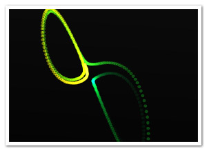
Chaos theory used to be a subject that interested me a lot in high school for some reason, and when looking at the subject, you can’t skim past Strange Attractors and, in particular, the famous Lorenz Attractor. An important aspect of what this system is showing, is that small changes in the initial state of a complex dynamical system can result in large and unexpected differences on a larger scale (commonly known as the butterfly effect). In this example for instance, changing the initial position just a little, will at first seem to converge with the trajectory of the original position. In later stages, however, it will diverge more and more. Plenty of that can be read in literature, and it’s beyond my scope here. The demo doesn’t really allow you to play around with that either, it only shows the trajectories for the constants in the equations. It’s mainly there for aesthetical reasons, and to give a source code example (right-click on the demo, you know the drill).

Anyway, I thought I’d just enlighten you on how to bring these babies to the screen. Why on earth would anyone even want to put them on a screen? Well, for some reason, I find them beautiful :D But perhaps more important, if you’re looking for complex, unpredictable, non-repeating, but pattern-like movements, you might just end up using differential equations (I’m thinking smoke, turbulence, adding milk to coffee…). Play around with it, and see what you can come up with.

In the case of the Lorenz attractor, the equation goes like this:
dx/dt = σ(y-x)
dy/dt = x(ρ-z)-y
dz/dt = xy-βz

In practice, this means that over an infinitisimal amount of time (dt), the variables x, y and z will change by the respective left-hand side of the equation. Of course, in programming, we’ll have to approximate the infinitisimal character. We’ll work in steps of time, instead. Obviously, smaller steps will be more correct. Let’s rework the equation just a tiny bit, replacing dt with our time step:

dx = σ(y-x)*timestep
dy = (x(ρ-z)-y)*timestep
dz = (xy-βz)*timestep

So afterwards, we just add dx, dy, and dz to x, y, and z respectively, and we have the next position in the trajectory! σ, ρ, and β are constants that will influence the attractor. By changing these values, there will be three possible situations: the trajectory will converge towards one point, diverge towards infinity, or will endlessly seem to be attracted around a set of points without ever repeating itself, in which case we have a chaotic system going.

And that’s it! Complexity doesn’t need to be complex at all :) Checkout the demo or the source to see the implementation.