Introduction

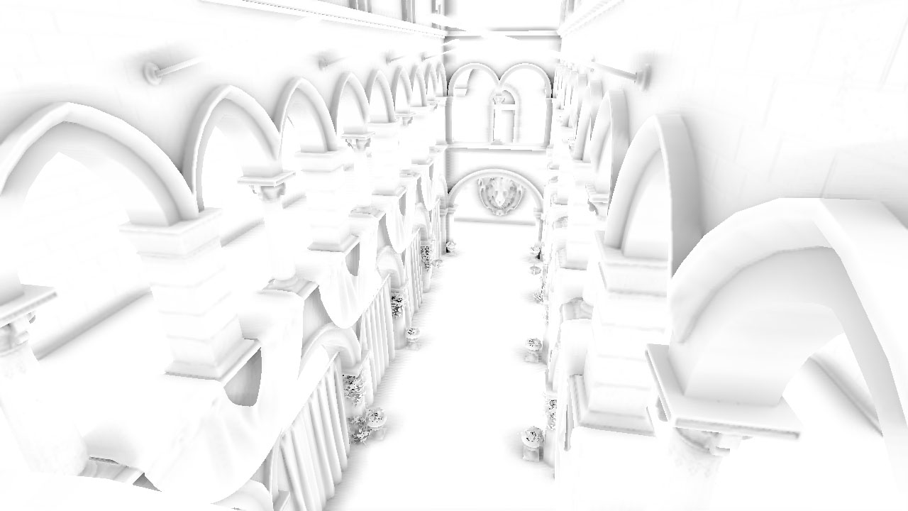
Image-space horizon-based ambient occlusion [HBAO] is a technique introduced by NVidia (Louis Bavoil et al.) in 2008. I recommend checking out the following resources to find out exactly how the algorithm works, this post will build on it further:

• ShaderX7 – Image-Space Horizon-Based Ambient Occlusion (by Louis Bavoil & Miguel Sainz)
• The original Siggraph paper (by Louis Bavoil, Miguel Sainz & Rouslan Dimitrov)
• Siggraph presentation
• Horizon-Based Ambient Occlusion using Compute Shaders

The ShaderX7 book in particular offers a well-explained detailed approach to the problem.
Before I continue, I’d like to extend my gratitude to Louis Bavoil for taking the time to review this article and giving some insightful tips on how to improve the shader.

A recap

Roughly, HBAO works by raymarching the depth buffer, and doing this in a number of equiangular directions across a circle in screen-space.

For the derivations, all points and vectors are expressed in spherical coordinates relative to the eye space basis. The azimuth angle rotates about the negated eye space Z-axis and the elevation angle is relative to the XY plane. This is a bit different to the common way of defining the polar angle, which is usually relative to the main axis, but the approach serves us well. The elevation angle is the only angle that will be of much interest to us, since the azimuthal integration will be handled entirely by marching in the different directions.

With each raymarch step, the line between the sample point and the centre point is considered. Each time the elevation angle is larger than the previous maximum, a new chunk of occluding geometry has been found. We add in the occlusion for the arc-segment between the last two found horizon vectors and weigh it with a distance function.

Note that the horizon angle is measured with respect to the plane parallel to the XY view plane, and therefore a tangent vector needs to be taken into consideration, with its angle relative to the same plane. This yields the following equation, as noted in ShaderX7:

For the derivation and other implementation details, please refer to the source material. It will be useful as I’ll explain the differences in the implementation I did for Helix.

The Helix approach

With respect to this article, the most important aspect of the original paper is that it uses eye-space as a basis for spherical coordinates, which is where this post will differ. While we’ll still use eye-space as a basis for our positions and vectors in the shader, for the derivations we’ll express the spherical coordinates relative to the normal vector and the tangent plane. Both changes will result in a leaner and, more importantly, trig-less approach. Here’s the previous figure reimagined:

Which will result in a similar equation, without involving :

We’ll take some liberties with the attenuation function, approximating it piecewise (see original). In practice, this means we define it to be constant between two adjacent horizon vectors, using the value at the furthest sample point. Furthermore, since we don’t snap to texel centres, we don’t need to make tangent adjustments as in the original. Focusing on the inner integral, we get:

Making the following observation, we can make our lives a lot easier:

This allows us to rewrite any occurence of as a simple dot product. Using the piecewise approximation for , the equation then becomes:

[Update]

One thing I forgot to mention that needs to be taken into account is the case when the angle extends 90 degrees:

In this case, the occlusion should be total, but the dot product with the normal would result in the wrong angle. This is actually a limitation of working in screen-space, where marching in 2D does not match a marching in 3D due to overlap. What we need to do is test the angle with the tangent: if , we simply do not have proper data in the direction we’re interested in: it could be completely occluded, or not at all. Personally, I find picking “half-occluded” works best in this case.

Some more implementation details

As with SSAO, to reduce banding artefacts, the orientations of all the sample directions should be rotated randomly per pixel. Helix’s approach takes one similar to Crytek’s original SSAO algorithm, using a 4×4 ‘dither’ texture containing the 2D rotation factors which is indexed so that it becomes tiled 1:1 over the screen. To assure an even distribution, rather than going for random angles, I instead used 16 evenly spaced angles between 0 and with being the amount of raymarching directions.
Furthermore, the dither texture also contains a jitter factor, which we’ll use to offset the starting position to reduce banding artefacts. This is similar to the original, with some nuances to play nice with the way view space positions are reconstructed in Helix. As per Louis Bavoil’s suggestion, introducing an extra sample closer to the center of the kernel creates more interesting contact occlusions. In my approach, both are combined by jittering the ray’s start position between the closest neighbour and the first sample size.
Using dithering obviously introduces a lot of noise. Performing a depth-dependent 4×4 box blur afterwards will remove this while making sure every pixel always has contributions from the same sample directions. Some implementations rotate the directions entirely randomly (non-tiled) and blur heavily, but I feel this tends to create what I can only describe as “static AO clouding”: you can see a static AO pattern moving along with the camera. Other implementations like to combine 4×4 dithering and heavy blurring, but personally I like to retain some of the higher frequency occlusions.

Subtle normal-based occlusion

Regarding the normals, the source recommends using face normals which can be derived from the depth buffer. However, I simply use the per-pixel normals that are stored in the deferred renderer’s normal buffer. While this can introduce artefacts, the use of a bias angle largely cancels them out while still adding some normal-based occlusion.

Comparison

Below, you can see a comparison between this HBAO approach and traditional SSAO using similar settings and sample count.

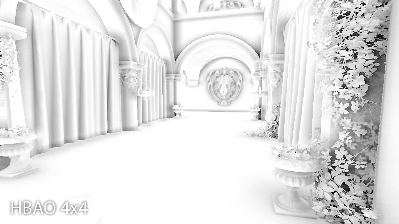
HBAO (4×4 samples)

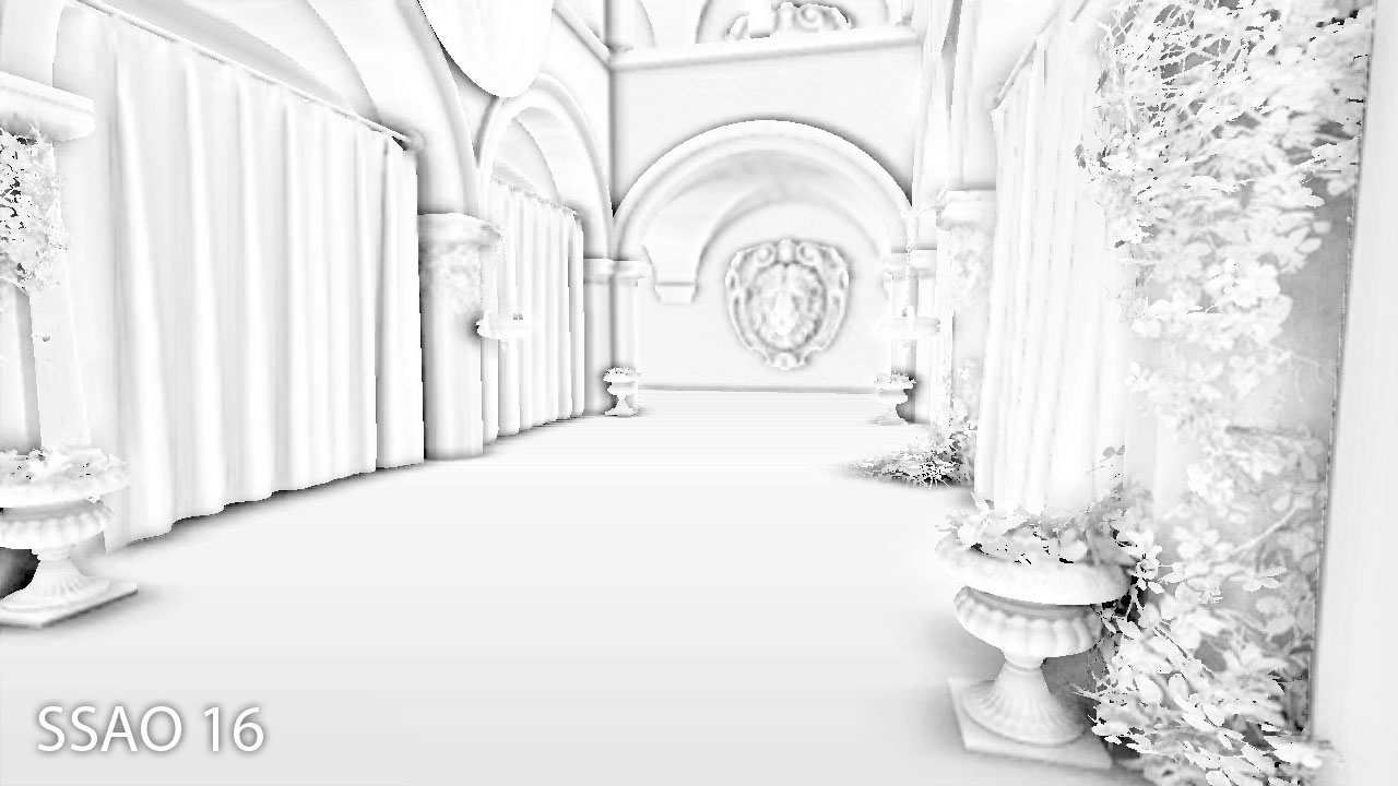
SSAO (16 samples)

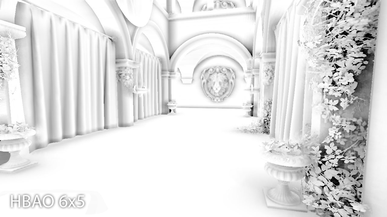
HBAO (6×5 samples)

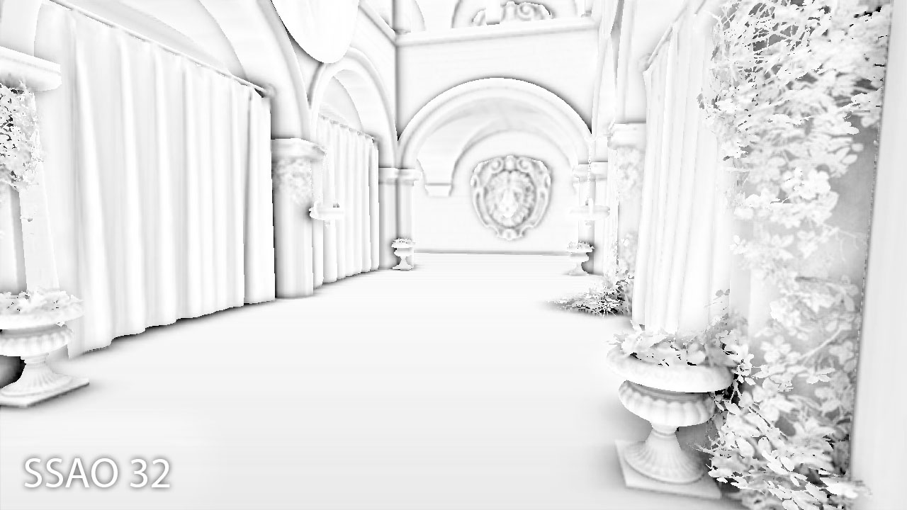
SSAO (32 samples)

Notice how there’s less over-occlusion, especially near discontinuities (for example between the curtain and floor) while some details are handled more correctly (such as the creases in the curtain to the right). Even with a relatively small amount of samples, the improvements are remarkable. I did boost the parameters on both, violating my own rules, but purely for illustrational purposes!

Example shader

I guess no one will be happy without some sample code. I can’t publish the entire Helix code (mainly because it’s a pretty inefficient mess right now) but I can show the shaders for the ambient occlusion step. The rest (blur shaders, etc) are default fare. All code is in HLSL Shader Model 5 for DirectX 11.

• Vertex shader
• Fragment shader

Conclusion

And that’s it! I hope this post was useful looking into different AO techniques. Any questions, comments, corrections, … are more than welcome!